Description of the solutions

The GRACE and GRACE-FO missions

The GRACE (Gravity Recovery and Climate Experiment; Tapley et al., 2004; Tapley et al., 2019) and GRACE-FO (GRACE Follow-On; Chen et al., 2022; Landerer et al., 2020) satellite missions have, since 2002, provided monthly estimates of variations in the Earth’s gravity field and of mass redistributions on its surface or at depth. These redistributions include mass changes in ice sheets, movements of water masses linked to hydrological cycles, and displacements of mantle masses associated with glacial isostatic adjustment and earthquakes. The GRACE and GRACE-FO missions consist of twin satellites equipped with a Star Camera Assembly (SCA), an accelerometer (ACC), GPS receivers, and K-band microwave transmitters (K-Band Ranging or KBR). The KBR data are processed as the relative velocity between the satellites, known as the K-Band Range-Rate (KBRR). In addition to the GRACE/-FO Level 1B data mentioned above, normal equations derived from satellite laser ranging (SLR) are added, providing a good estimate of the long-wavelength components of the geopotential at low harmonic degrees. Combining GRACE/-FO data with SLR data allows for the calculation of Earth’s geopotential anomalies by inverting the normal equations derived from satellite orbit adjustments. This inversion yields the coefficients of the spherical harmonic decomposition of the geopotential, known as the Level 2A (L2A) solution. As part of the constrained solution developed by CNES, the stabilization of the inversion relies on the use of a singular value decomposition (SVD) truncated at high orders which have an extremely low signal-to-noise ratio (Lemoine et al., 2026). This approach introduces an additional constraint that reduces the noise level compared to a classical inversion based on a Cholesky decomposition (see here). Under these conditions, the application of Gaussian or DDK spatial filters (Kusche et al., 2009) is not required for the extraction of geophysical signals of interest for Earth observation, as the SVD truncation already optimizes the signal-to-noise ratio.

Files description

The time series of the GRACE CNES SVD solutions is provided in the form of spherical harmonic coefficients up to degree and order 90, excluding degree 0 (8,280 coefficients). The C00 coefficient still appears in the file with a value of 1.0, but should not be taken into account when using the solutions (see example below). These solutions are obtained by constraining the low degrees of the field using SLR data, through an inversion via Singular Value Decomposition (SVD) (more details are available here). The solutions are distributed in ASCII files, with the coefficients sorted according to the extended GRACE format, which is an extension of the original format of the GRACE gravity models (document GR-GFZ-FD-001 GRACE 327-732 (v1.1), November 27, 2003, available here), sorted in ascending order of degree and order. An example file is provided below.

Solution Quality Metrics

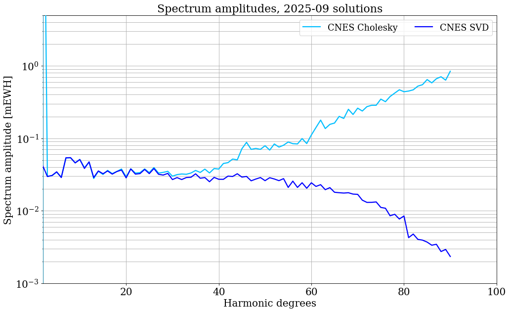
Just as with Cholesky solutions, spectral amplitude serves as a relevant quality metric for SVD solutions. The impact of SVD stabilization is reflected in the amplitude of the solution spectrum (see Figure 1), where the increase in the spectrum observed starting at degree 30 in the Cholesky solutions does not appear. SVD stabilization also attenuates the noise peaks associated with the orbit’s resonance harmonics (multiples of 15), which are clearly visible in the Cholesky solutions (see the example in the figure below).

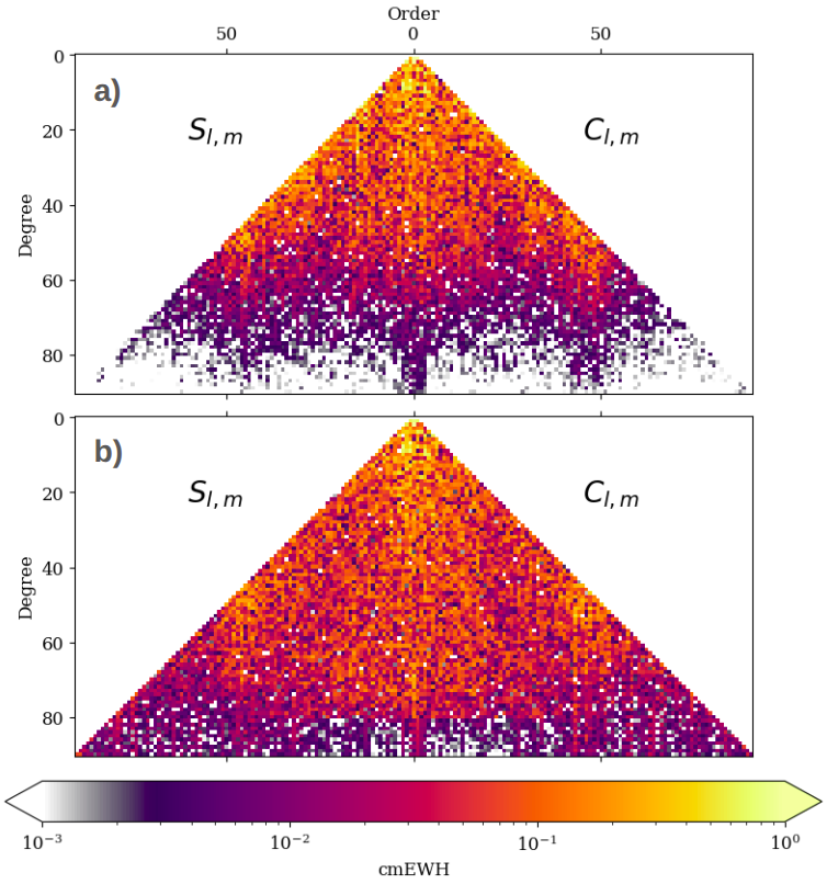
Due to the polar orbit of the GRACE/-FO satellites, instrumental errors and errors in the underlying geophysical models (tides, ocean-atmosphere aliasing) accumulate and correlate along the satellite track, resulting in strong anisotropic noise in the unconstrained geopotential solutions, which manifests as the characteristic streaks in these missions. SVD stabilization reduces the noise level, as shown in Figure 2, which displays the amplitude of the SVD solution coefficients, comparable to those of the filtered Cholesky solution. By comparing the coefficient trees of the filtered Cholesky solution with the SVD solution, we can observe that the amplitude of the coefficients is greater for the SVD solution at degrees higher than 60, which results in a higher-resolution signal once gridded.

Using the solutions

In order to use these solutions, it is necessary to express the gravitational potential at every point on Earth. The Earth’s gravitational potential is expressed as follows:

Where r, φ, and λ are, respectively, the radius, latitude, and longitude of the considered point, C_lm and S_lm are the harmonic coefficients of the solution, G is the universal gravitational constant, M is the mass of the Earth, a is the Earth’s equatorial radius, P̅_lm is the associated Legendre function of degree l and order m.

The solutions of the GRACE/-FO geopotential allow us to track variations in mass on the Earth’s surface, particularly water masses, since the solutions are generally expressed as variations in a thin layer of water on its surface. In this case, the previous equation becomes, when calculated up to a maximum degree L_max:

Where:

– ΔH_W(φ, λ) is the equivalent water height at latitude φ and longitude λ,
– a is the Earth’s average radius,
– ρ_E is the average Earth density,
– ρ_w is the water density,
– k_l is the Load Love Number (LLN) at any harmonic degree l,
– Y̅_lm are the Legendre polynomial functions for any degree l and order m, in complex notation,
– ΔC̅_lm are the increments, relative to a reference gravitational solution, of the complex spherical harmonic coefficients of the solution.

More details about the method can be found in Ditmar (2018).

Dataset identifier

10.24400/170160/SAGSA_GGM_SVD_1MONTH_RL0005

Characteristics

	Product type	Stokes coefficients
	Format	ASCII files
	License	(CCBY)
	Start of production	GRACE: 01/04/2002 | GRACE-FO: 01/05/2018
	End of production	GRACE: 01/05/2017 | GRACE-FO: Still producing
	Coverage	Global
	Coverage type	Spherical harmonics
	Spatial resolution	Maximum degree: 90
	Time resolution	Monthly solutions
	Mission(s)	GRACE | GRACE-FO
	Instrument(s) / Captor(s)	Star Camera Assembly (SCA), Accelerometer (ACC), K-Band Ranging (KBR), GPS, SLR

Bibliography

- Chen et al., 2022; Ditmar, 2018; Dobslaw et al., 2017; Kusche et al., 2009; Landerer et al., 2020; Lemoine et al., 2026; Tapley et al., 2004, 2019
- Chen, J., Cazenave, A., Dahle, C., Llovel, W., Panet, I., Pfeffer, J., & Moreira, L. (2022). Applications and Challenges of GRACE and GRACE Follow-On Satellite Gravimetry. Surveys in Geophysics, 43(1), 305‑345. https://doi.org/10.1007/s10712-021-09685-x
- Ditmar, P. (2018). Conversion of time-varying Stokes coefficients into mass anomalies at the Earth’s surface considering the Earth’s oblateness. Journal of Geodesy, 92(12), 1401‑1412. https://doi.org/10.1007/s00190-018-1128-0
- Dobslaw, H., Bergmann-Wolf, I., Dill, R., Poropat, L., Thomas, M., Dahle, C., Esselborn, S., König, R., & Flechtner, F. (2017). A new high-resolution model of non-tidal atmosphere and ocean mass variability for de-aliasing of satellite gravity observations : AOD1B RL06. Geophysical Journal International, 211(1), 263‑269. https://doi.org/10.1093/gji/ggx302
- Kusche, J., Schmidt, R., Petrovic, S., & Rietbroek, R. (2009). Decorrelated GRACE time-variable gravity solutions by GFZ, and their validation using a hydrological model. Journal of Geodesy, 83(10), 903‑913. https://doi.org/10.1007/s00190-009-0308-3
- Landerer, F. W., Flechtner, F. M., Save, H., Webb, F. H., Bandikova, T., Bertiger, W. I., Bettadpur, S. V., Byun, S. H., Dahle, C., Dobslaw, H., Fahnestock, E., Harvey, N., Kang, Z., Kruizinga, G. L. H., Loomis, B. D., McCullough, C., Murböck, M., Nagel, P., Paik, M., … Yuan, D.-N. (2020). Extending the Global Mass Change Data Record : GRACE Follow-On Instrument and Science Data Performance. Geophysical Research Letters, 47(12), e2020GL088306. https://doi.org/https://doi.org/10.1029/2020GL088306
- Lemoine, J.-M., Bourgogne, S., Gégout, P., Reinquin, F., Marty, J.-C., Mercier, F., Loyer, S., Bruinsma, S., & Balmino, G. (2026). 22 years of time-variable gravity field determination from GRACE and GRACE Follow-On : The CNES/GRGS RL05 solution. Journal of Geodesy, 100(2), 20. https://doi.org/10.1007/s00190-026-02040-1
- Tapley, B. D., Bettadpur, S., Watkins, M., & Reigber, C. (2004). The gravity recovery and climate experiment : Mission overview and early results. Geophysical Research Letters, 31(9), n/a-n/a. https://doi.org/10.1029/2004gl019920
- Tapley, B. D., Watkins, M. M., Flechtner, F., Reigber, C., Bettadpur, S., Rodell, M., Sasgen, I., Famiglietti, J. S., Landerer, F. W., Chambers, D. P., Reager, J. T., Gardner, A. S., Save, H., Ivins, E. R., Swenson, S. C., Boening, C., Dahle, C., Wiese, D. N., Dobslaw, H., … Velicogna, I. (2019). Contributions of GRACE to understanding climate change. Nature Climate Change, 9(5), 358‑369. https://doi.org/10.1038/s41558-019-0456-2