CNES SAGSA GRACE/-FO Level 3 Ensemble


Ensemble approach
The GRACE and GRACE-FO satellite missions continuously measure the Earth’s gravitational field and its evolution over time (Tapley et al., 2004, Landerer et al., 2020, respectively). With a spatial resolution of a few hundred kilometers and a temporal resolution that is generally monthly, these missions provide a unique view of global-scale mass redistribution, enhancing our understanding of water (Pfeffer et al., 2022) and energy (Meyssignac et al., 2019) cycles in a changing climate.
To accurately track variations in water mass in the oceans, hydrosphere, and cryosphere, Level 2 GRACE/-FO data must be corrected to:
- Remove non-water-related effects, such as Earth deformations resulting from deglaciation or earthquakes.
- Compensate for the limitations of satellites, which are not very sensitive—or not sensitive at all—to variations in gravity on a very large spatial scale.
- Reduce errors associated with anisotropic noise or signal leakage near coastlines (“leakage” effect).
The PANIS software applies these corrections and generates the SAGSA L3 ensemble, based on the ensemble approach described by (Blazquez et al., 2018). This method combines several L2 products and models using current best practices to produce robust surface water mass anomalies, while systematically estimating the uncertainties associated with the processing and post-processing choices for GRACE and GRACE-FO data.
Unlike the COST-G combined solution, which provides Level 2 geopotential products, SAGSA focuses on Level 3 surface water mass anomalies. The SAGSA dataset is thus an essential tool for research in hydrology, oceanography, and glaciology, providing both the water mass anomalies themselves and the uncertainties associated with their estimation.
Processing steps
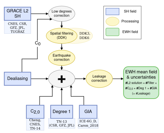
The SAGSA ensemble is based on Level 2 GRACE/-FO products generated by five processing centers, which estimate anomalies in the Earth’s gravitational potential in the form of Stokes coefficients (i.e., in the spherical harmonic basis). It includes solutions provided by JPL (GRACE-FO, 2024), CSR (NASA/JPL, 2023), GFZ (Dahle et al., 2018), the ITSG (Kvas et al., 2019), and the CNES (J.-M. Lemoine et al., 2026).
These coefficients are subject to several sources of error and limitations, which require corrections during various post-processing steps.
- The GRACE and GRACE-FO satellites orbit the Earth’s center of mass and are therefore not sensitive to the movement of the geocenter. They cannot therefore be used to estimate first-order Stokes coefficients. The monthly values of the degree 1 coefficients are estimated in the SAGSA v2.1 dataset based on the method of Sun et al., 2016, using input data from three different processing centers (e.g., JPL, CSR, GFZ).
- GRACE and GRACE-FO measurements are also insensitive to low-degrees components of the gravity field, particularly the C20 and C30 coefficients. In this ensemble, the C20 (full time series) and C30 (after May 2016 only) coefficients, estimated by the five processing centers, are replaced by more robust SLR measurements from three different data centers (Cheng et al., 2013 ; J. Lemoine & Reinquin, 2017 ; Loomis et al., 2019).
- To extract mass variations associated with the redistribution of water within the hydrosphere, the ocean, and the cryosphere, GRACE and GRACE-FO data must be corrected for ongoing viscoelastic Earth deformations caused by past deglaciation. Two different GIA models are used here (Caron et al., 2018 ; Peltier et al., 2018). No correction for the Little Ice Age (LIA) is applied.
- The Stokes coefficients are affected by systematic correlated errors, easily identifiable in the spatial domain as characteristic vertical stripes. To reduce this anisotropic noise, decorrelation filters, known as DDK filters (Kusche et al., 2009), are applied to the GRACE solutions in two different orders (DDK3 and DDK6), corresponding to two levels of filtering.
The combination of five processing centers, three geocenter models, three obliquity values (C20, C30), two GIA models, and two filtering levels results in a set of 180 solutions. Additional corrections are applied identically to all members of the set:
- A seismic correction to remove co-seismic deformations from major earthquakes.
- A “leakage” correction (Lecomte et al., 2025) is applied near the coasts to correctly relocate mass anomalies initially located in the ocean toward nearby land. This correction is based on a model of the coastal ocean that uses, for each time step, the average of the corresponding ocean basin.
- Reconstruction of ocean dealiasing models using the GAB model derived from AOD1B RL06 (Dobslaw et al., 2017).
- Gravitational potentials are corrected to account for the total mass of atmospheric water vapor expressed in C0 GAA, in order to ensure mass conservation on a global scale (Chen et al., 2019).
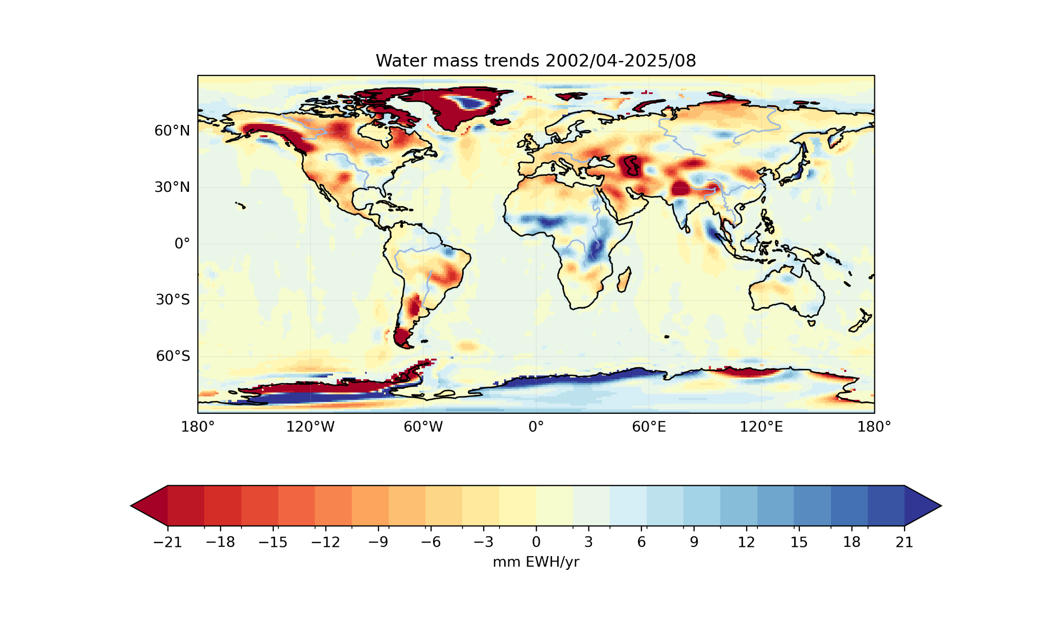
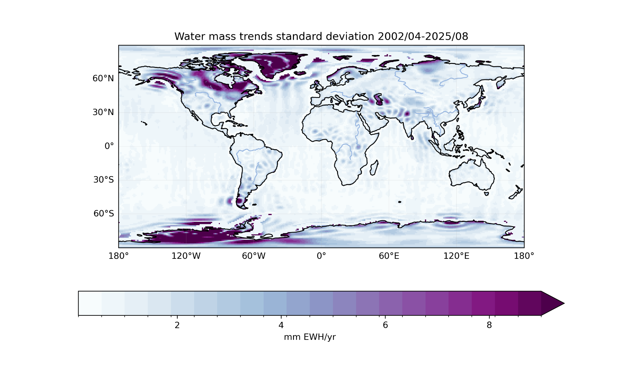
This approach, illustrated in Figure 2, provides a set of 180 solutions consisting of monthly surface mass anomalies gridded onto a regular global grid of 1° × 1°, expressed in equivalent water height.
Files description
The gravimetry dataset is available in NetCDF files and in zarr format.
The file contains the combined solutions and corrections, stored in the “water_thickness” or “lwe_thickness” variable, including:
- Analysis center (e.g., CNES, GFZ, ITSG, JPL, CSR),
- Filter (e.g., DDK3, DDK6),
- Seismic correction,
- GIA correction (e.g., Caron, Peltier),
- Leakage correction,
- C20 and C30 solution (e.g., Loomis, Lemoine, Chen),
- Geocenter solution (e.g., TN13a, b, or c)
Users will also find as variables a ‘land_mask’, the total water content of the atmosphere as ’water_atmosphere_eq’ and the list of names for each element of the combination. For more details on the correction methods and the data used, please refer to the PANIS ATBD (see below).
Ensemble Quality Metrics
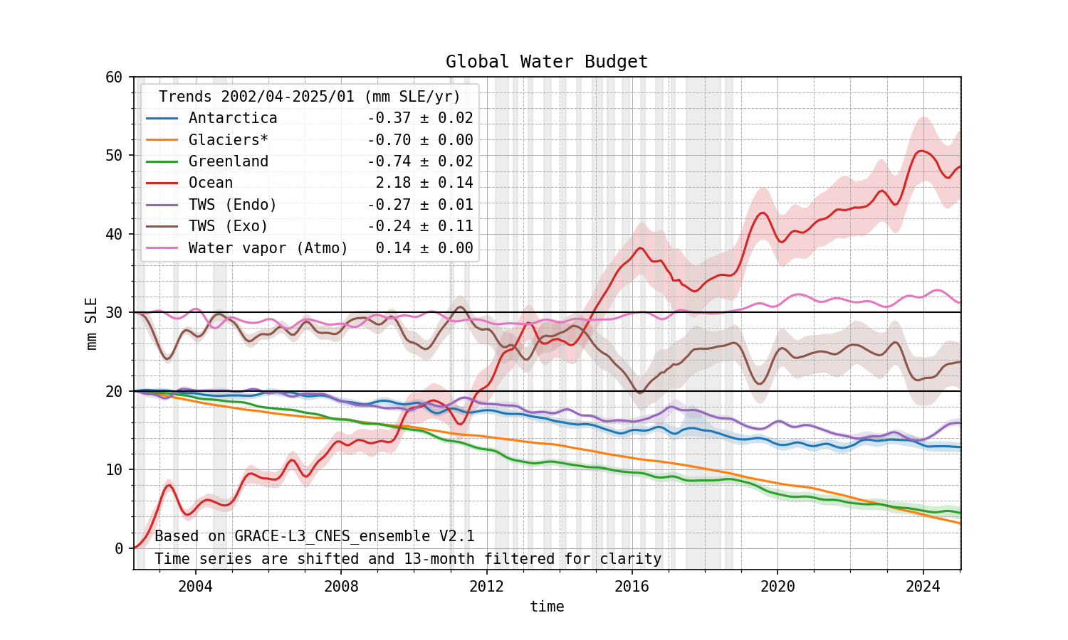
An example of a system-wide quality metric is the balance of contributions to changes in the barystatic level. The sum of the contributions from the various sources, as illustrated in Figure 3, must equal the changes in sea level to ensure the conservation of mass in the Earth system.
The example presented for the V2.1 dataset shows that this balance is correctly maintained, confirming the proper conservation of mass within the dataset. Other quality metrics are described in greater detail in the PANIS ATBD.
Using the solutions
To use the gravimetry dataset, users are encouraged to use the tools from the Python xarray library, which are best suited for handling NetCDF and .zarr files.
WARNING: The full versions of the dataset can be very large (over 20 GB) and may overload your system. It is strongly recommended that you process the full dataset using a computing cluster.
A simplified version of the dataset containing only its mean and one-sigma uncertainty is available here.
Dataset identifier
10.24400/170160/SAGSA_ENSEMBLE_1MONTH_EXPERT_V2.1
Characteristics
| Product type | Monthly equivalent water height grids ensemble | |
| Format | NetCDF4 and .zarr files | |
| License | (CCBY) | |
| Start of production | GRACE: 01/04/2002 | GRACE-FO: 01/05/2018 | |
| End of production | GRACE: 01/05/2017 | GRACE-FO: Still producing | |
| Coverage | -180° – 180° ; -90° – 90° | |
| Coverage type | Global | |
| Spatial resolution | 1°x1° | |
| Time resolution | Monthly grids | |
| Mission(s) | GRACE | GRACE-FO | |
| Instrument(s) / Captor(s) | Star Camera Assembly (SCA), Accelerometer (ACC), K-Band Ranging (KBR), GPS, SLR |
Recommended references
- ATBD PANIS: Download link
- Blazquez et al., 2018
Version table for the complete ensemble
| Name | Version | Publication Date | Time Coverage | DOI | Product User Manual | How to Cite |
|---|---|---|---|---|---|---|
| L3_CNES_SAGSA_ENSEMBLE_1MONTH_expert_V2.1 | 2.1 | 05/03/2026 | 2002-04 – 2025-08 | 10.24400/170160/SAGSA_ENSEMBLE_1MONTH_EXPERT_V2.1 | In preparation (estimated publication date: second half of 2026) | A. Boughanemi, J. Pfeffer, A. Blazquez, H. Lecomte, N. Lalau, R. Fraudeau, and E. Pellereau. Sagsa graceensemble expert, 2025a. URL https://geodes.cnes.fr/projects/l3_cnes_sagsa_ensemble_1month_expert/. |
Bibliography
- (Blazquez et al., 2018; Caron et al., 2018; Chen et al., 2019, 2022; Cheng et al., 2013; Dahle et al., 2018; Dobslaw et al., 2017; GRACE-FO, 2024; Kusche et al., 2009; Kvas et al., 2019; Landerer et al., 2020; Lecomte et al., 2025; J. Lemoine & Reinquin, 2017; J.-M. Lemoine et al., 2026; Loomis et al., 2019; Meyssignac et al., 2019; NASA/JPL, 2023; Peltier et al., 2018; Pfeffer et al., 2022; Sun et al., 2016; Tapley et al., 2004, 2019)
- Blazquez, A., Meyssignac, B., Lemoine, J., Berthier, E., Ribes, A., & Cazenave, A. (2018). Exploring the uncertainty in GRACE estimates of the mass redistributions at the Earth surface : Implications for the global water and sea level budgets. Geophysical Journal International, 215(1), 415‑430. https://doi.org/10.1093/gji/ggy293
- Caron, L., Ivins, E. R., Larour, E., Adhikari, S., Nilsson, J., & Blewitt, G. (2018). GIA Model Statistics for GRACE Hydrology, Cryosphere, and Ocean Science. Geophysical Research Letters, 45(5), 2203‑2212. https://doi.org/https://doi.org/10.1002/2017GL076644
- Chen, J., Cazenave, A., Dahle, C., Llovel, W., Panet, I., Pfeffer, J., & Moreira, L. (2022). Applications and Challenges of GRACE and GRACE Follow-On Satellite Gravimetry. Surveys in Geophysics, 43(1), 305‑345. https://doi.org/10.1007/s10712-021-09685-x
- Chen, J., Tapley, B., Seo, K.-W., Wilson, C., & Ries, J. (2019). Improved Quantification of Global Mean Ocean Mass Change Using GRACE Satellite Gravimetry Measurements. Geophysical Research Letters, 46(23), 13984‑13991. https://doi.org/10.1029/2019GL085519
- Cheng, M., Tapley, B. D., & Ries, J. C. (2013). Deceleration in the Earth’s oblateness. Journal of Geophysical Research: Solid Earth, 118(2), 740‑747. https://doi.org/10.1002/jgrb.50058
- Dahle, C., Flechtner, F., Murböck, M., Michalak, G., Neumayer, H., Abrykosov, O., Reinhold, A., & König, R. (2018). GRACE Geopotential GSM Coefficients GFZ RL06 (Version 6.0, p. 3 Files) [Application/octet-stream,application/octet-stream,application/octet-stream]. GFZ Data Services. https://doi.org/10.5880/GFZ.GRACE_06_GSM
- Dobslaw, H., Bergmann-Wolf, I., Dill, R., Poropat, L., Thomas, M., Dahle, C., Esselborn, S., König, R., & Flechtner, F. (2017). A new high-resolution model of non-tidal atmosphere and ocean mass variability for de-aliasing of satellite gravity observations : AOD1B RL06. Geophysical Journal International, 211(1), 263‑269. https://doi.org/10.1093/gji/ggx302
- GRACE-FO. (2024). GRACE-FO Level-2 Monthly Geopotential Spherical Harmonics JPL Release 6.3 [Jeu de données]. NASA Physical Oceanography Distributed Active Archive Center. https://doi.org/10.5067/GFL20-MJ063
- Kusche, J., Schmidt, R., Petrovic, S., & Rietbroek, R. (2009). Decorrelated GRACE time-variable gravity solutions by GFZ, and their validation using a hydrological model. Journal of Geodesy, 83(10), 903‑913. https://doi.org/10.1007/s00190-009-0308-3
- Kvas, A., Behzadpour, S., Ellmer, M., Klinger, B., Strasser, S., Zehentner, N., & Mayer‐Gürr, T. (2019). ITSG‐Grace2018 : Overview and Evaluation of a New GRACE‐Only Gravity Field Time Series. Journal of Geophysical Research: Solid Earth, 124(8), 9332‑9344. https://doi.org/10.1029/2019JB017415
- Landerer, F. W., Flechtner, F. M., Save, H., Webb, F. H., Bandikova, T., Bertiger, W. I., Bettadpur, S. V., Byun, S. H., Dahle, C., Dobslaw, H., Fahnestock, E., Harvey, N., Kang, Z., Kruizinga, G. L. H., Loomis, B. D., McCullough, C., Murböck, M., Nagel, P., Paik, M., … Yuan, D.-N. (2020). Extending the Global Mass Change Data Record : GRACE Follow-On Instrument and Science Data Performance. Geophysical Research Letters, 47(12), e2020GL088306. https://doi.org/https://doi.org/10.1029/2020GL088306
- Lecomte, H., Blazquez, A., fourest, sebastien, meyssignac, benoit, pfeffer, julia, boughanemi, alexandre, & pellereau, eric. (2025). Leakage Corrections for GRACE Level-3 Solutions and Associated Induced Uncertainties. IAG Proceedings 2025.
- Lemoine, J., & Reinquin, F. (2017). Processing of SLR observations at CNES. Newsletter EGSIEM, 3.
- Lemoine, J.-M., Bourgogne, S., Gégout, P., Reinquin, F., Marty, J.-C., Mercier, F., Loyer, S., Bruinsma, S., & Balmino, G. (2026). 22 years of time-variable gravity field determination from GRACE and GRACE Follow-On : The CNES/GRGS RL05 solution. Journal of Geodesy, 100(2), 20. https://doi.org/10.1007/s00190-026-02040-1
- Loomis, B. D., Rachlin, K. E., & Luthcke, S. B. (2019). Improved Earth Oblateness Rate Reveals Increased Ice Sheet Losses and Mass-Driven Sea Level Rise. Geophysical Research Letters, 46(12), 6910‑6917. https://doi.org/https://doi.org/10.1029/2019GL082929
- Meyssignac, B., Boyer, T., Zhao, Z., Hakuba, M. Z., Landerer, F. W., Stammer, D., Köhl, A., Kato, S., L’Ecuyer, T., Ablain, M., Abraham, J. P., Blazquez, A., Cazenave, A., Church, J. A., Cowley, R., Cheng, L., Domingues, C. M., Giglio, D., Gouretski, V., … Zilberman, N. (2019). Measuring Global Ocean Heat Content to Estimate the Earth Energy Imbalance. Frontiers in Marine Science, 6(432). https://doi.org/10.3389/fmars.2019.00432
- NASA/JPL. (2023). GRACE-FO Level-2 Monthly Geopotential Spherical Harmonics CSR Release 6.2 (RL06.2) [Jeu de données]. NASA Physical Oceanography Distributed Active Archive Center. https://doi.org/10.5067/GFL20-MC062
- Peltier, W. R., Argus, D. F., & Drummond, R. (2018). Comment on “An Assessment of the ICE-6G_C (VM5a) Glacial Isostatic Adjustment Model” by Purcell et al. Journal of Geophysical Research: Solid Earth, 123(2), 2019‑2028. https://doi.org/10.1002/2016JB013844
- Pfeffer, J., Cazenave, A., & Barnoud, A. (2022). Analysis of the interannual variability in satellite gravity solutions : Detection of climate modes fingerprints in water mass displacements across continents and oceans. Climate Dynamics, 58(3‑4), 1065‑1084. https://doi.org/10.1007/s00382-021-05953-z
- Sun, Y., Riva, R., & Ditmar, P. (2016). Optimizing estimates of annual variations and trends in geocenter motion and J2 from a combination of GRACE data and geophysical models. Journal of Geophysical Research: Solid Earth, 121(11), 8352‑8370. https://doi.org/https://doi.org/10.1002/2016JB013073
- Tapley, B. D., Bettadpur, S., Watkins, M., & Reigber, C. (2004). The gravity recovery and climate experiment : Mission overview and early results. Geophysical Research Letters, 31(9), n/a-n/a. https://doi.org/10.1029/2004gl019920 Tapley, B. D., Watkins, M. M., Flechtner, F., Reigber, C., Bettadpur, S., Rodell, M., Sasgen, I., Famiglietti, J. S., Landerer, F. W., Chambers, D. P., Reager, J. T., Gardner, A. S., Save, H., Ivins, E. R., Swenson, S. C., Boening, C., Dahle, C., Wiese, D. N., Dobslaw, H., … Velicogna, I. (2019). Contributions of GRACE to understanding climate change. Nature Climate Change, 9(5), 358‑369. https://doi.org/10.1038/s41558-019-0456-2