Description of the solutions

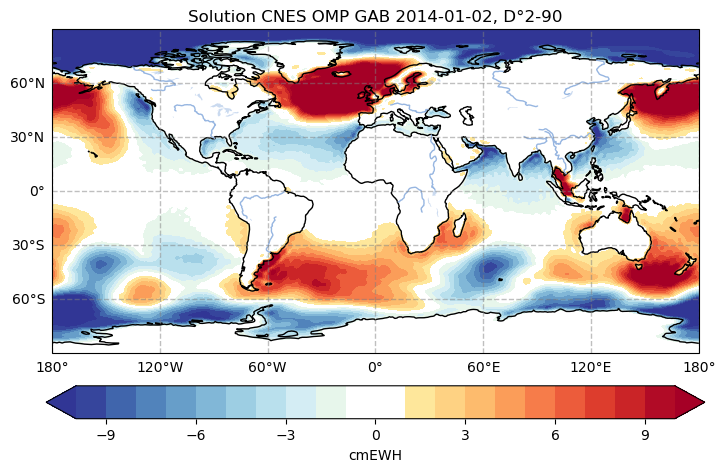
The ERA-Interim and TUGO dealiasing products enable the estimation of spatial and temporal variations in the gravitational potential of the atmosphere and the ocean in 3D. The mean value of the original grids, calculated over a 10-year period (2001–2010), was subtracted from the time series, so that the OMP dealiasing products represent only the time-varying component of the gravitational interaction between the atmosphere and ocean masses. Geopotential anomalies due to ocean mass redistributions were calculated using the TUGO barotropic model, which estimates the oceanic response to ERA-Interim atmospheric forcing, taking into account variations in pressure and wind speed every 3 hours.

The oceanic dealiasing model was calculated by Florent Lyard (LEGOS/CNRS). The response of the solid Earth to this time-varying oceanic potential was accounted for using Love numbers kp (see here). The 10-days dealiasing models are obtained by averaging the 3-hour products, taking into account the arcs used for the production of the geopotential solutions. An example of a 10-days dealiasing model is shown in Figure 1.

Files description

The time series of ocean dealiasing models is provided in the form of spherical harmonic coefficients up to degree and order 90, excluding degrees 0 and 1 (8,277 coefficients). The coefficients for degrees 0 and 1 appear in the files with a value of zero. The solutions are distributed in ASCII files, with the coefficients sorted according to the extended GRACE format, which is an extension of the original GRACE gravity model format (document GR-GFZ-FD-001 GRACE 327-732 (v1.1), November 27, 2003, available here), sorted in ascending order of degree and order. An example file is provided below.

Using the solutions

In order to use these solutions, it is necessary to express the gravitational potential at every point on Earth. The Earth’s gravitational potential is expressed as follows:

Where r, φ, and λ are, respectively, the radius, latitude, and longitude of the considered point, C_lm and S_lm are the harmonic coefficients of the solution, G is the universal gravitational constant, M is the mass of the Earth, a is the Earth’s equatorial radius, P̅_lm is the associated Legendre function of degree l and order m.

Generally, the gravitational potential is expressed at the Earth’s surface. Since the models are based on the GRACE/-FO geopotential solutions, they must be expressed in the same way—that is, generally as variations in a thin layer of water on the Earth’s surface. In this case, the previous equation becomes, when calculated up to a maximum degree L_max:

Where:

– ΔH_W(φ, λ) is the equivalent water height at latitude φ and longitude λ,
– a is the Earth’s average radius,
– ρ_E is the average Earth density,
– ρ_w is the water density,
– k_l is the Load Love Number (LLN) at any harmonic degree l,
– Y̅_lm are the Legendre polynomial functions for any degree l and order m, in complex notation,
– ΔC̅_lm are the increments, relative to a reference gravitational solution, of the complex spherical harmonic coefficients of the solution.

More details about the method can be found in Ditmar (2018).

Dataset identifier

10.24400/170160/SAGSA_GGM_GAB_10DAYS_RL0005

Characteristics

	Product type	Stokes coefficients
	Format	ASCII files
	License	(CCBY)
	Start of production	01/04/2002
	End of production	01/05/2017
	Coverage	Global
	Coverage type	Spherical harmonics
	Spatial resolution	Maximum degree: 90
	Time resolution	10-days models
	Mission(s)	None
	Instrument(s) / Captor(s)	None